Painting credits: Vincent van Gogh - Van Gogh self-portrait (1889)
13th June 2022
What is Neural Style Transfer?
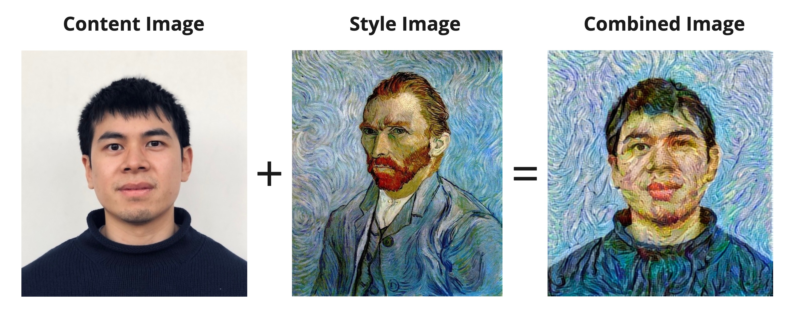
Ever wanted to see how Van Gogh would paint your portrait? Neural Style Transfer (NST) is a method that aims to blend the style of one image (the style image) with the contents of another (the content image), allowing the user to give an artistic touch to the image of their choice. This technology isn’t particularly new and has been around for a while (see the original paper by Gatys, et al., 2015), so there are definitely more sophistated ways to approached this problem now. Nevertheless, learning to build NSTs is extremely fun and has helped develop my understanding of convolutional neural networks.
NST isn’t perfect, and admittedly the results are often quite bad as you don’t have perfect control over the model’s behaviour. This generally requires a lot of experimentation to learn which image combinations, model configurations, etc. work best. But after many hours of trial and error, I think I got some pretty good results. I passed some of my own photographs with a specific painting into the NST model with the hope of transferring the artistic style from the painting to my photograph. I'll present my best results below first, and then more information about how NST works for those interested will come after.
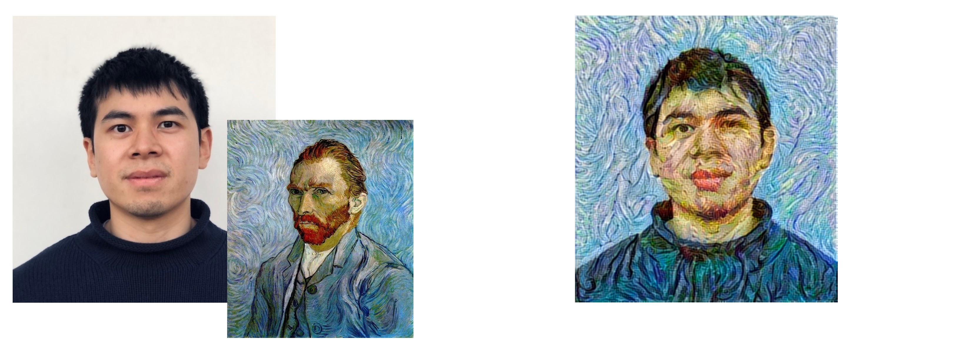
Painting credits: Vincent van Gogh - Van Gogh self-portrait (1889)
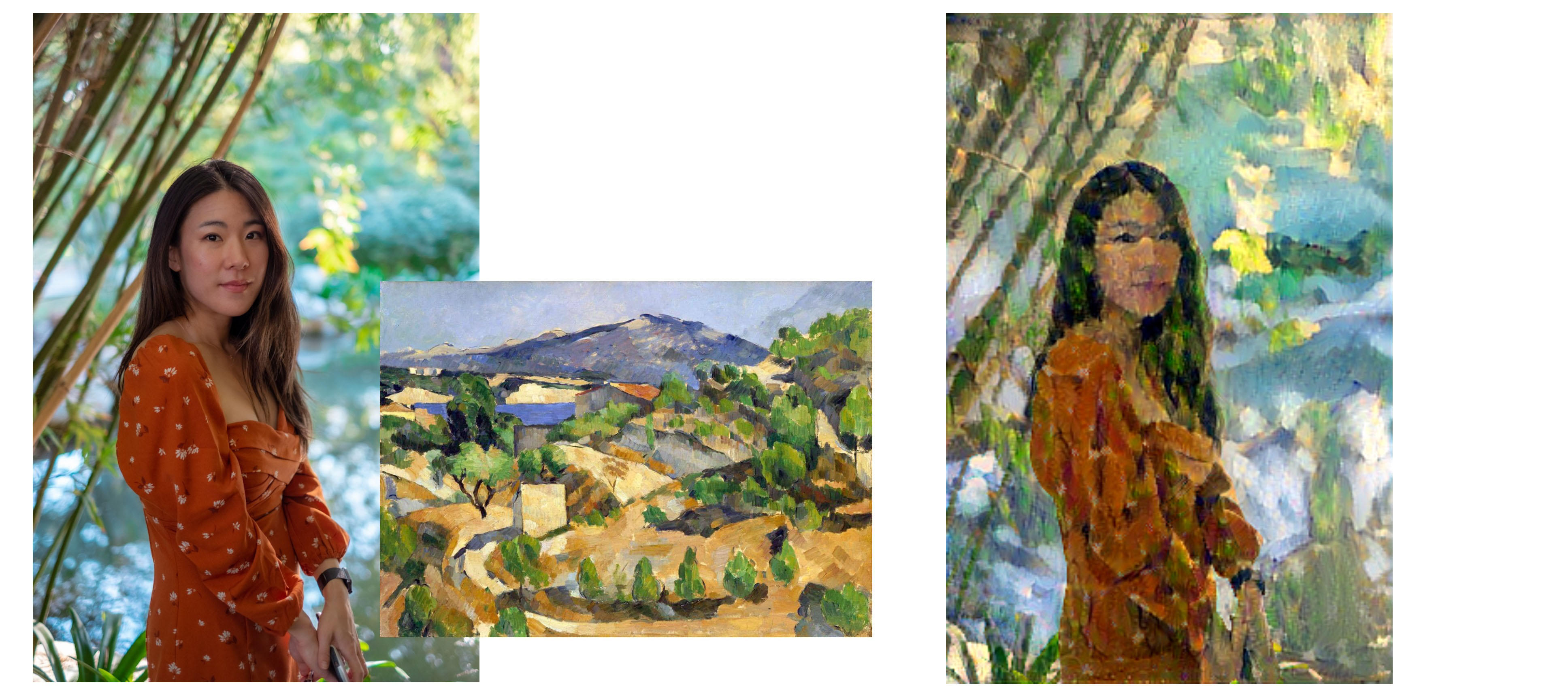
Painting credits: Paul Cézanne - Mountains in Provence L'Estaque (1880)
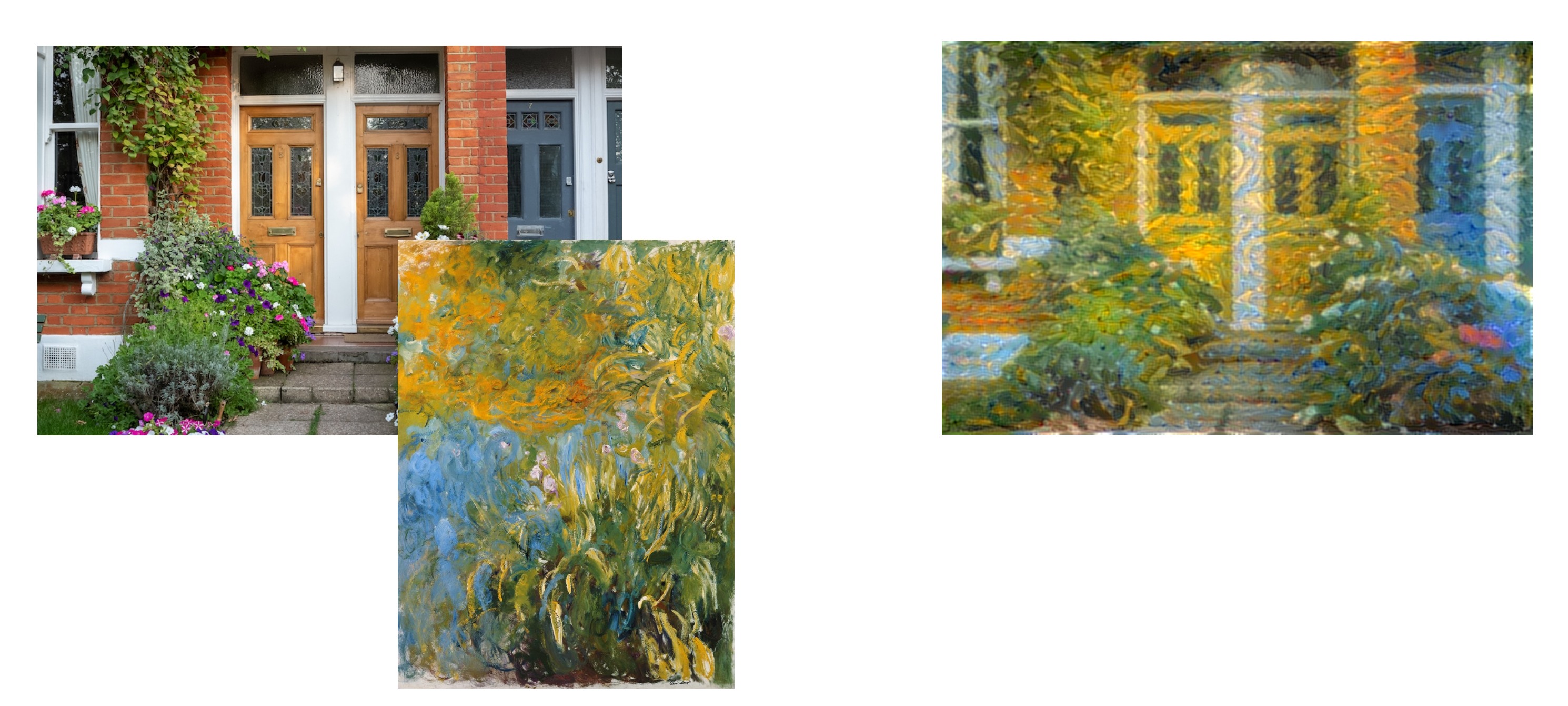
Painting credits: Claude Monet - Irises by the Pont (1917)
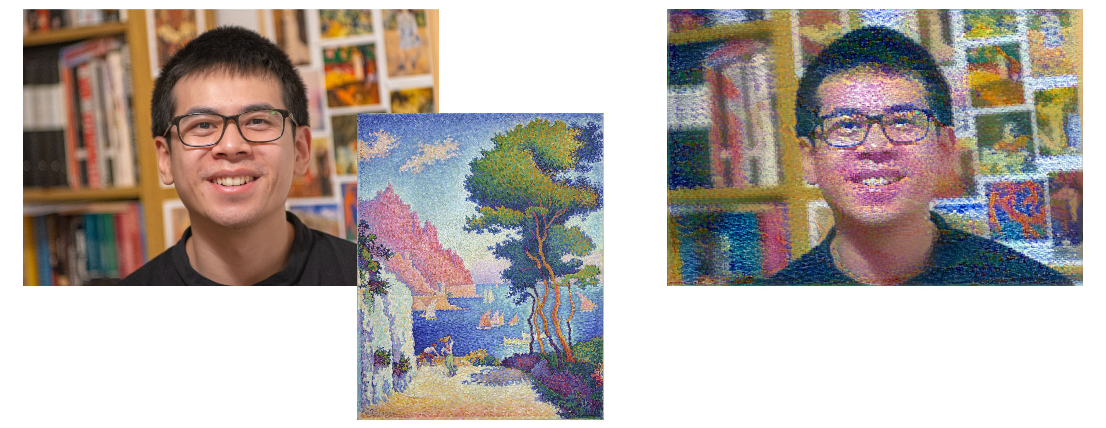
Painting credits: Paul Signac - Capo di Noli (1898)
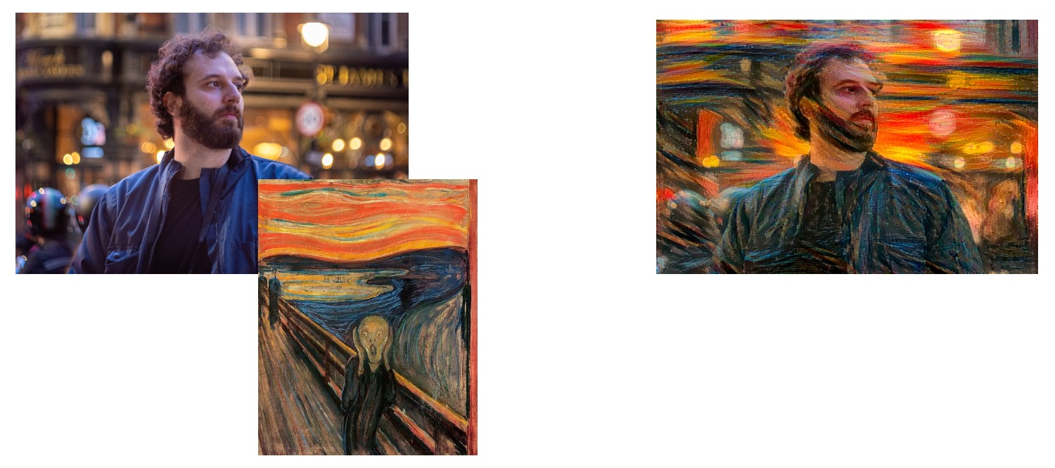
Painting credits: Edvard Munch, The Scream (1893)
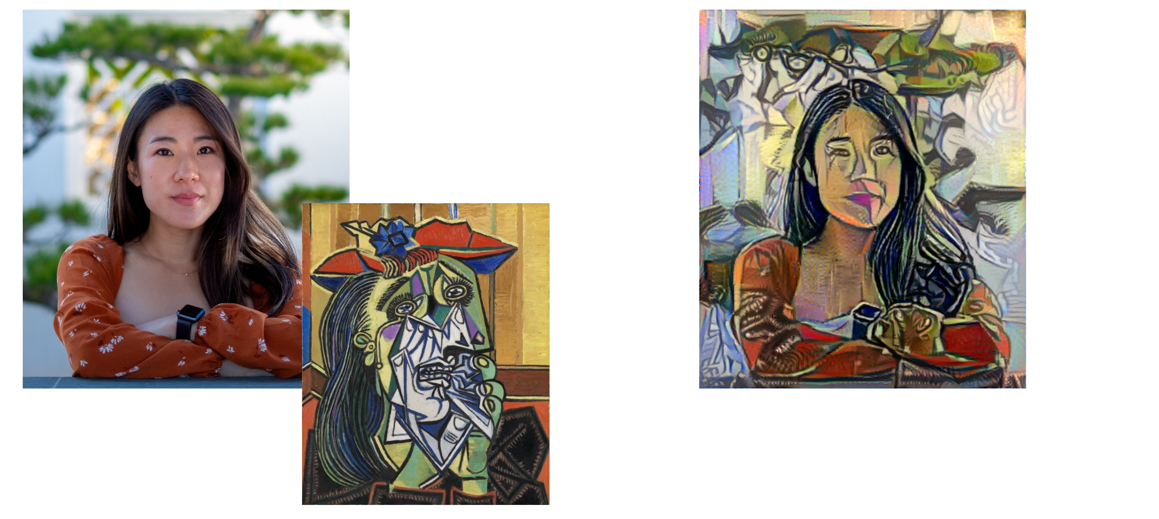
Painting credits: Pablo Picasso - The Weeping Woman (1937)
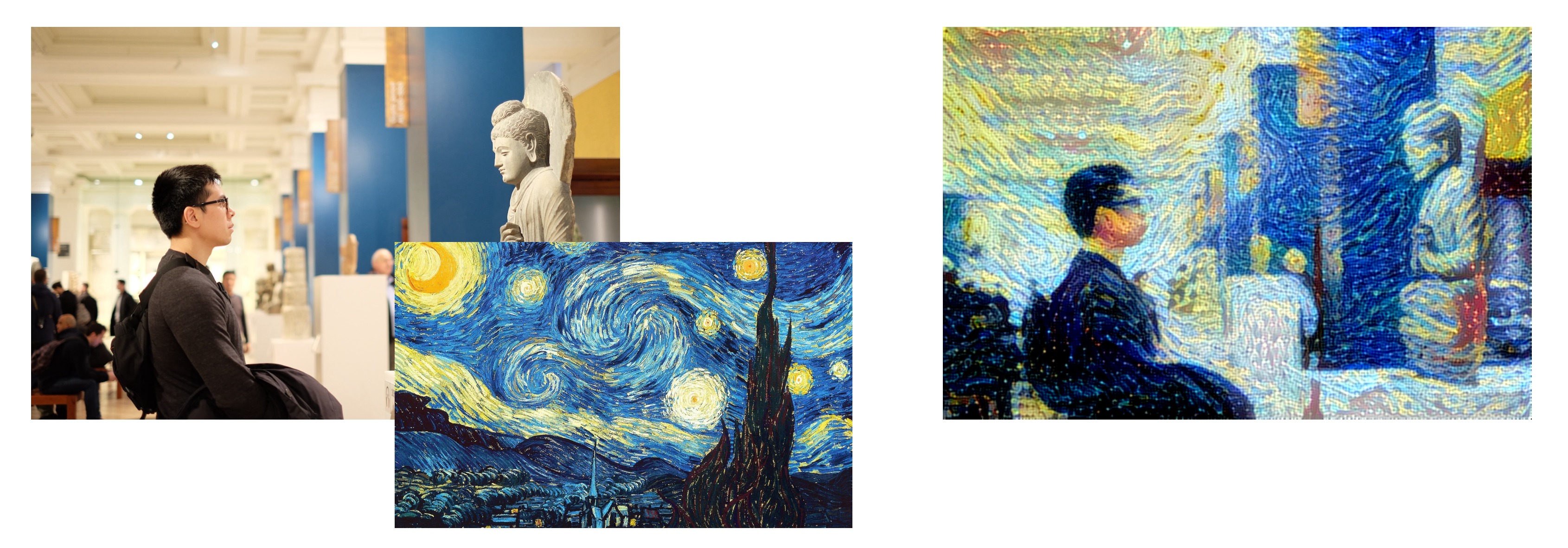
Painting credits: Vincent van Gogh - The Starry Night (1889)
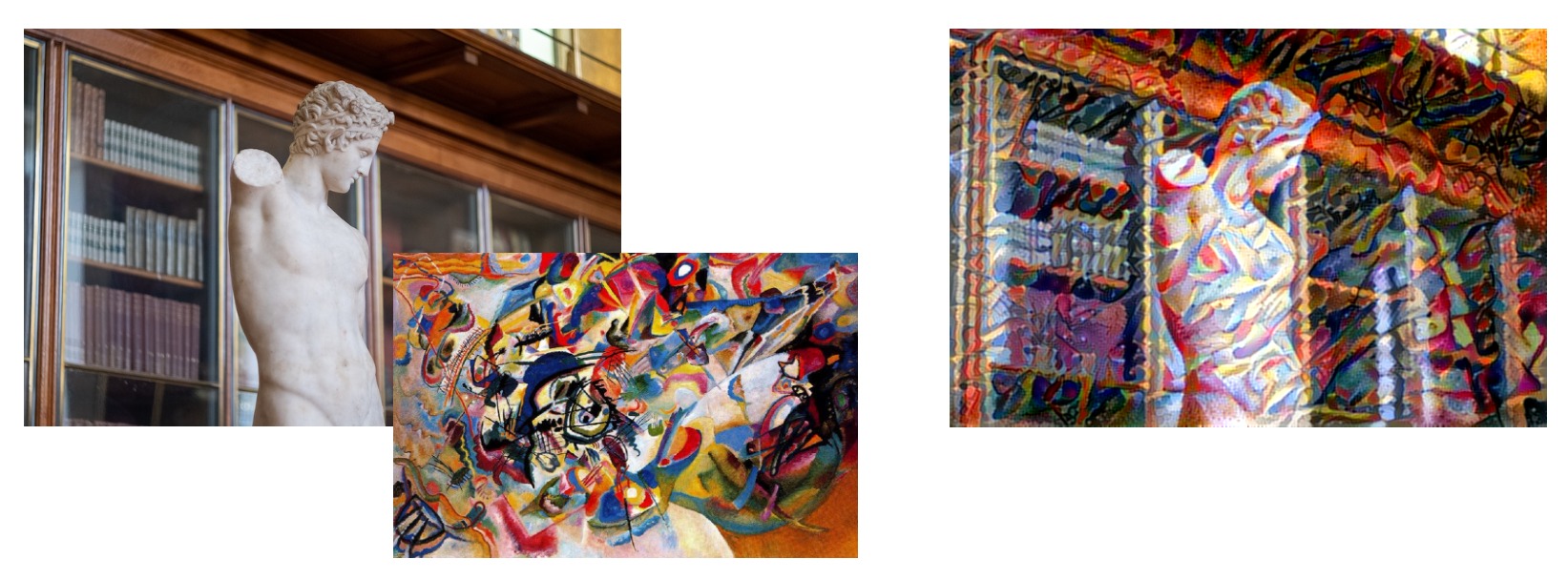
Painting credits: Wassily Kandinsky, Composition VII (1913)
Quick note about alternative methods
As you may know, there are other areas of deep learning that aim to generate images that could have been leveraged for this problem, for example:
- Variational Autoencoders consist of an encoder and decoder model that aims to encode information about images in a generalised latent space, wherein a point in that latent space can be decoded into a new image.
- Diffusion Models are trained by iteratively increasing the Gaussian noise of the training data, with the aim of recovering the original image. The result is a model that should be able to denoise randomly sampled noise inputs into images that look like the training data.
- Generative Adversarial Networks (GANs) involves training two neural networks, a generator and discriminator, in competition with each other, wherein the generator’s primary goal is to “trick” the discriminator with newly generated images that look “real”.
However, these models aim to generate “completely new” images that resemble the original training images. This often requires large amounts of training data and computational resources. For example, if you wanted to build a model that can generate pictures of new Pokémon, you’ll need a several thousand images of Pokémon, at least one GPU, a very sophisticated model architecture and lots of time and patience to get the results you’re looking for.
NST reduces the complexity of this problem; instead of generating “completely new” images, it creates a combined image by extracting the style from a style image and blends it with the content image. The key advantage here is that it doesn’t require any training data and makes use of pre-trained neural networks that have already been trained to identify millions of different images, thus reducing time and effort.
NST overview
NST uses a pre-trained model, in this example we use ImageNet-VGG19 (VGG-19) (see Simonyan, et al. 2015 for more info). This is a convolutional neural network (CNN) model that has been trained to classify 14 million images belonging to 1000 different classes (more info about the ImageNet dataset here, and see Krizhevsky, et al. 2012 for further info on classification with CNNs). Note that you could technically use any pre-trained model trained on image data, we just happen to use VGG-19 here.
Using the pre-trained VGG-19 model removes the need to train a model from scratch, allowing us to leverage the knowledge that VGG-19 gained while learning to classify 1000 different object classes. This knowledge is embedded in the convolutional layers' filters, which can help identify key features of images at varying degrees of detail (such as shapes, colours, contrast, eyes, hands, wheels, etc.).
Here, we are simply taking a model that was trained on one task (image classification), and re-purposing it for another task (NST). This involves removing the classification head and using the intermediate layers to optimize a new loss function.
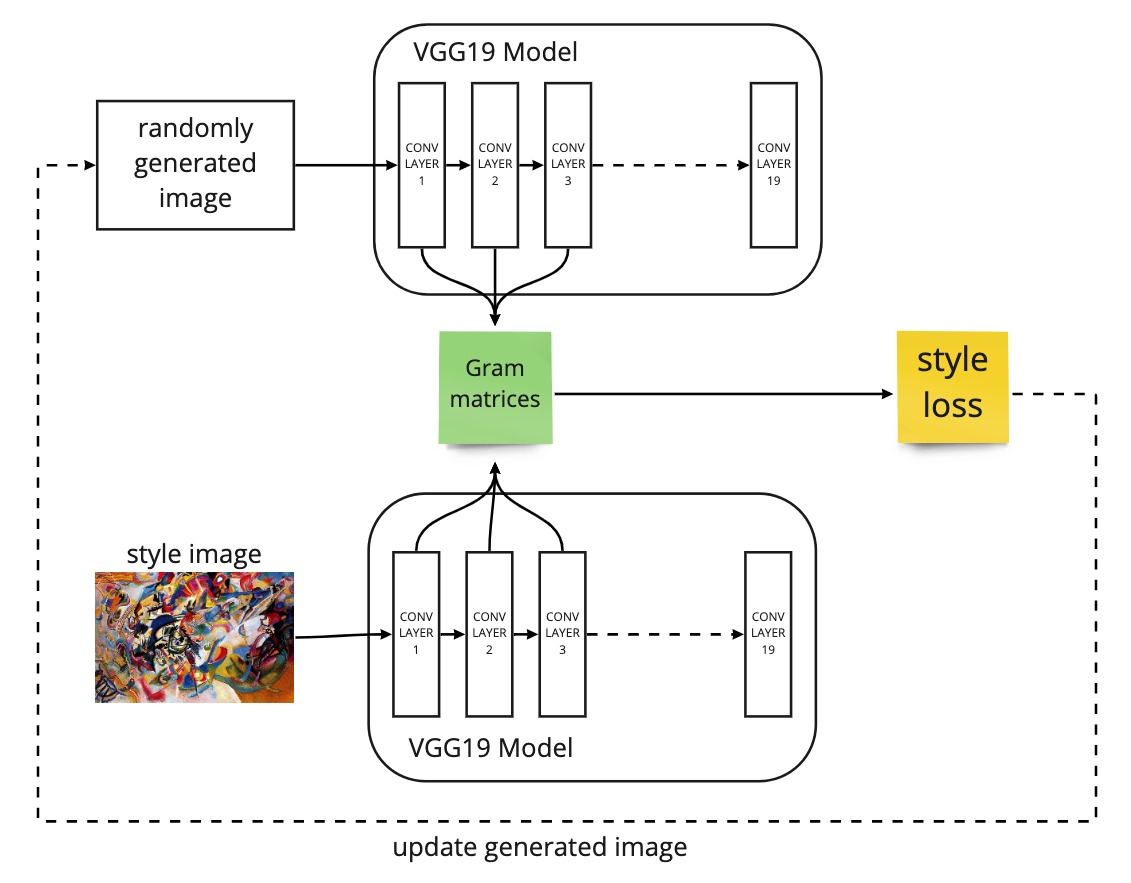
The NST model will start off with randomly generated pixels, acting as a placeholder for the combined image, and this will be compared against the style image and the content image via a unique loss function. This loss function comprises a weighted sum of 2 different losses:
- The content loss, which ensures the randomly generated image (combined image) contains the same content as the content image.
- The style loss, which ensures the randomly generated image (combined image) has the same general style as the style image.
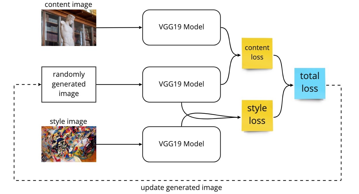
A diagram illustrating the architecture of neural style transfer.
Note that ordinarily, the loss function is minimised by the updating of model weights during backpropagation. However, with NST, the VGG19 weights are frozen, and the loss function is minimised by changing the pixel values of the combined image. In other words, the pixel values will be adjusted at each iteration to slowly produce a combined image that will minimise the loss function as a result of merging the style of one image and with the contents of another image.
Convolutional Neural Networks, Transfer Learning and VGG16
The fundamental building block of CNNs are the convolutional layers, where each layer develops a low-level understanding of the image via a series of filters. During training, the convolutional layers will automatically learn the most valuable filters to minimise its loss function for the training task. These filters help generate abstract feature maps that are activated by specific visual elements of an image.
For example, the lower-level layers contain abstract feature maps that highlight areas that tend to activate on lower-level details (such as vertical lines, curved lines, green pixels, etc.). When convolutional layers are stacked on top of each other, the higher-level layers will inevitably build on top of these lower-level feature maps and learn filters that activate on higher-level details (for example, identify shapes that look like eyes, flowers, clouds, chairs, etc.). Hint: lower-layers will contain style information and higher-layers will contain the content information.
For the classification task, the output of the final convolutional layer is a final feature map highlighting all the image’s key features, allowing the model to easily classify the image. (see Zeiler, et al. 2013 for visualising the behaviour of CNNs). In this case, the VGG-19 model does exactly that. It is made up of 16 convolutional layers (and 3 fully connected layers) that has been trained to classify 1000 object classes (e.g., table, car, cat, dog, etc.). As a result of this classification task, the network has developed rich feature representations for a wide range of images.
Therefore, each convolutional layer in the network can act as a complex feature extractor, whereby we can take the output of specific layers from the network to identify how well the model is merging the content and style image together. For example, the higher layer likely contains more generalised content information, while the low-mid layers contain lower-level details that align with the style information. See the image below for an illustrated example of this.
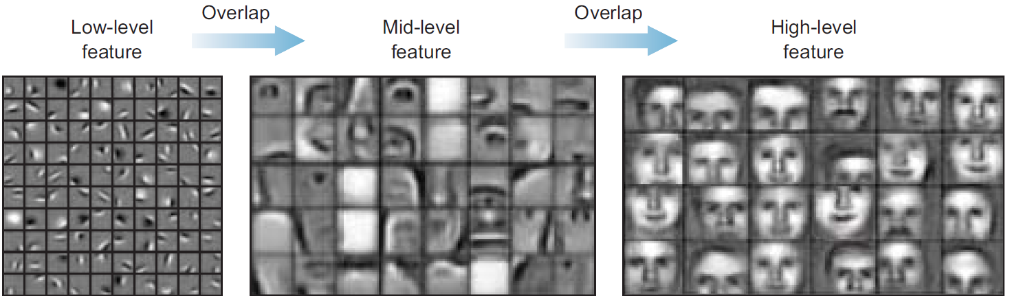
Image credits: Grokking Deep Learning for Computer Vision
Content Loss
If the scenes of two images look-alike (for example, a photo of a bus at a bus stop, and another photo of the same people taken in a different angle), the loss between these two images should be smaller than two images that have totally different scenes. Here, the content loss is not concerned about the minute details of the individual pixels. We want the content loss to penalise the combined image based on the presence of higher-level shapes and features such as the buildings, trees, or people in the combined image.
As described previously, when convolutional layers are stacked on top of each other, the higher-level layers tend to output abstract feature maps that highlight the higher-level features of images (i.e., identify the overall contents of images). If two images have the same contents, similar features should be highlighted by the higher layers.
Thus, for the content loss, we are most interested in the top-most convolution layer which will output feature maps containing the information about higher-level features of the images. So, the content loss is made of the mean squared error between these outputs.
To minimise this loss, the model will calculate the gradients from the loss and alter the pixel values of the generated image (remember the model weights are frozen!) such that the contents become closer and closer to that of the content image. This loss will ensure that the appropriate contents are captured in the final combined image.
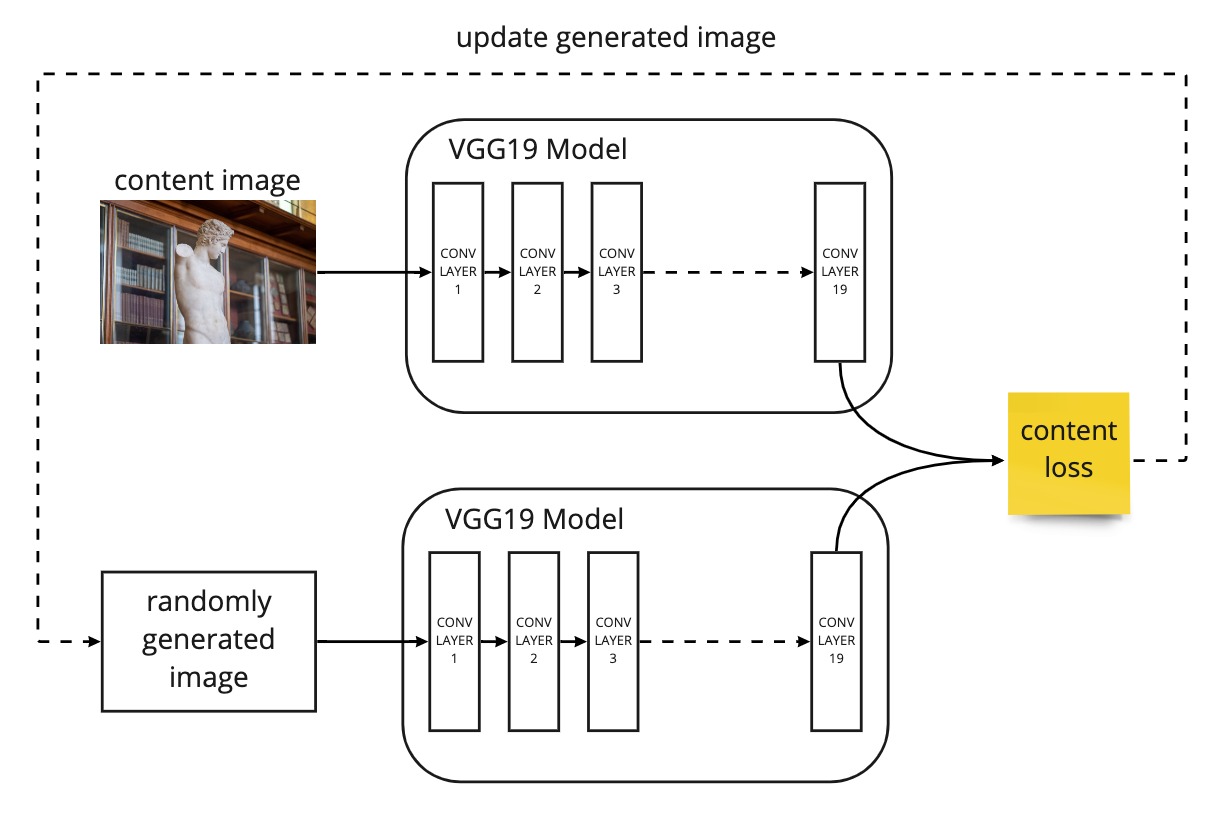
A diagram illustrating the intuition behind the content loss.
Style Loss
Like the content loss, the style loss ensures that the style of the style image is captured in the combined image. The aim here is to preserve the low-level details of the style image (like brush strokes, colour patterns, sharp edges, etc.) by extracting style information from the VGG-19 model. As mentioned previously, the higher layer are likely to extract more generalised content information, while the lower-intermediate layers extracts lower-level details that align with the style information. So, it makes sense to focus on outputs of the lower-intermediate layers.
Let’s illustrate this with a simple example. Suppose the VGG-19 network contains 3 convolutional filters that have learned to identify parts of the image that are coloured white, another vertical lines, and another brown. Each image will activate the corresponding feature maps at different areas depending on where the white colours, vertical lines and brown colours lie in the images.
See the image below, this is a simple representation of the feature maps for 3 different images on 3 different filters, where the darker red indicated larger activation.
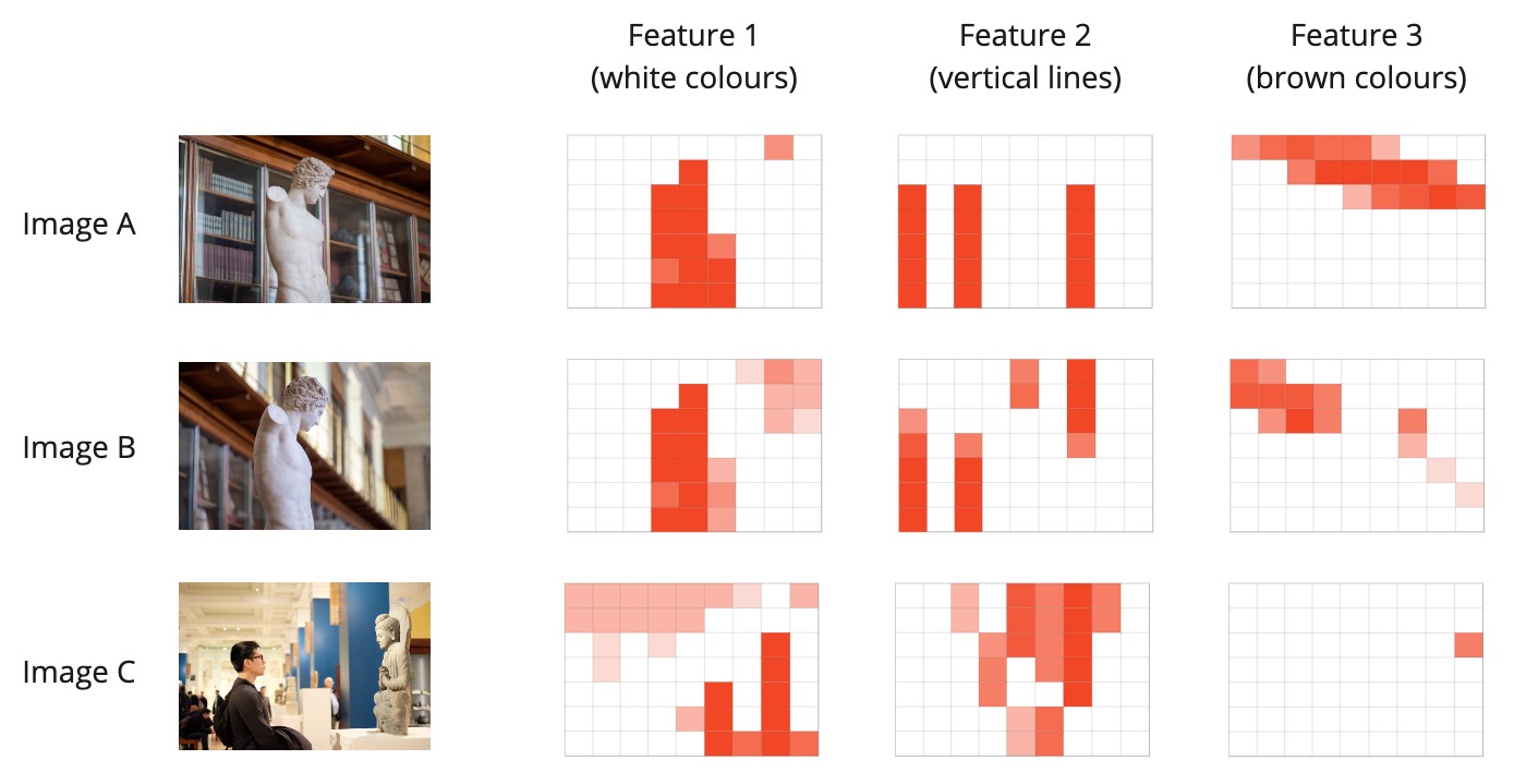
A simple diagram of the feature maps produced by Images A, B & C on specific filters.
We can see here that Images A & B are similar in style (both contain a white figure in the middle, brown colours are similarly placed in the background, etc.) but we can also see this by looking at the feature maps. You can see that the white and brown feature maps are strongly activated roughly around the same spatial points in Images A & B, but not in Image C. And conversely, the points at which the vertical line feature maps are activated in Image C are very different to those of Images A & B.
Gram Matrix
With this information, we can calculate something called the gram matrices for each layer of each image by flattening the output feature maps and calculating their dot products. By taking the dot products of the feature map activations, we can see how strongly or weakly correlated the features are in each layer.
See the image below, this shows the gram matrices for Image A, B & C and the 3 different feature maps (white colours, vertical lines, brown features colours).
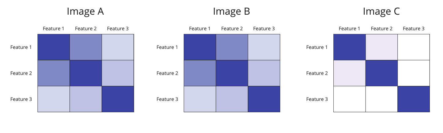
A simple diagram of gram matrices, representing the correlation between the feature maps per image.
The gram matrices show that Images A & B have very similar correlation patterns based on these 3 features, whilst the gram matrix of Image C is quite different. Even though the content of Images A & B may differ, their gram matrices are similar (i.e., they have white colours, vertical lines, and brown colours in roughly the same areas of the image). Thus, we can conclude that they have similar styles.
The gram matrix is effectively a way to interpret style information across the overall distribution of feature map activations per image per intermediate layer.
As such, the style loss can be defined as the root mean square difference between the gram matrices between the generated image and the style image of the intermediate layers. By trying to minimise the style loss between two images, you are essentially matching the distribution of features between the two images and trying to steer to generated image’s style to be closer that of the style image.
A diagram illustration the intuition behind the style loss.
Final Loss
Now that we have an understanding of the content loss and the style loss, we can see that the final loss is simple the weighted average of these two losses. You can control the amount of content and style imparted into the combined image by changing these weightings (see Gatys, et al. 2015 to understand the effects of changing such weights). Below shows the final model architecture indicating the layers that contribute to the style and content losses respectively.
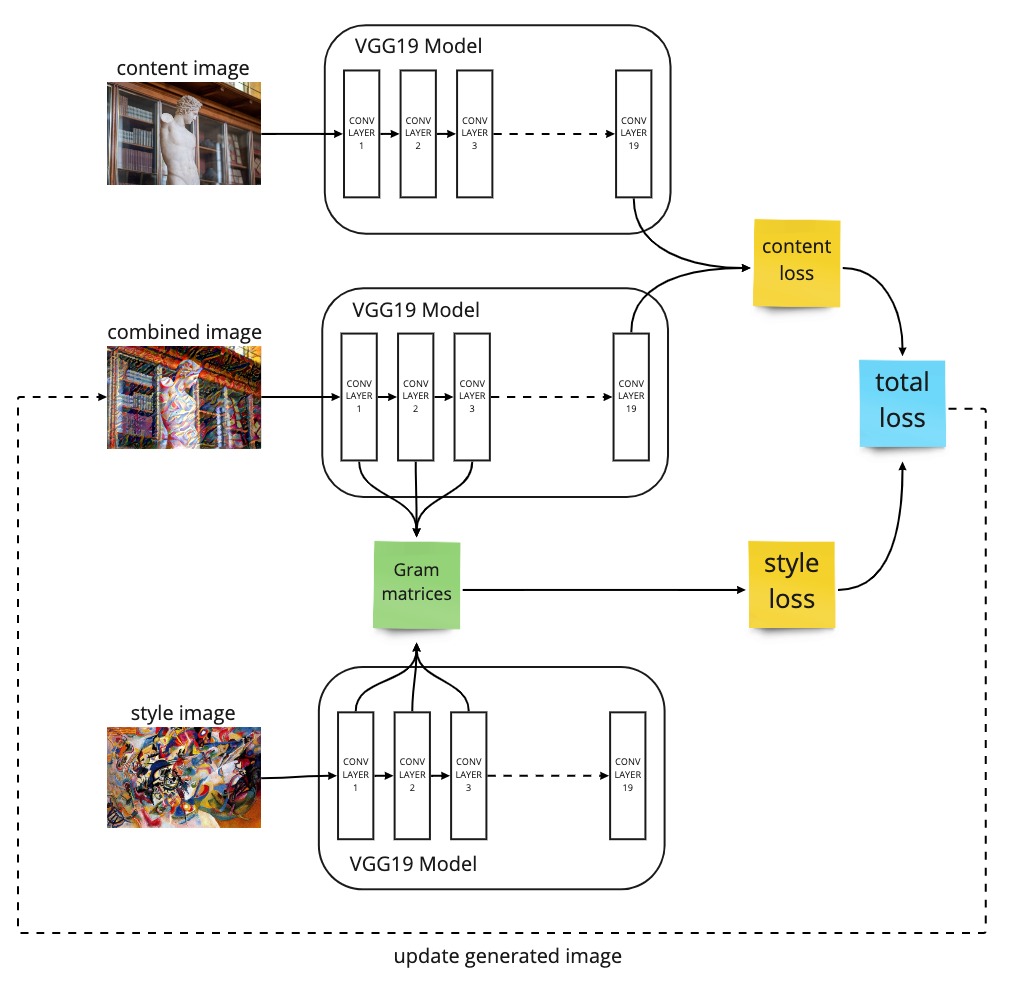
A simple diagram illustrating the entire neural style transfer architecture with the final loss function, made up of the style loss and content loss.
Conclusion
NST is a unique technique that allows us to merge the style of a style image with the contents of a content image by using a unique loss function that penalises the model for drifting too far from the contents and the artistic style of the images above.
However, NST is far from perfect, and as suggested in the beginning of this article, a lot of trial and error is required to get reasonable outputs. Most of the time, your results will be terrible. There are many ways to reconfigure this architecture for your needs. You can try changing the weighting parameters in the loss function, or select different layer combinations for the style and/or content loss, or try decaying the weight given to each layer in the style loss function to bias the model toward transferring finer or coarser style features. The more you experiment with this, the more of an intuition you'll develop around the type of image combinations that will be successful.
For those interested, my implementation of NST can be found in this GitHub repo. You’ll find that a simple Google search will very quickly return other code implementations of NST (most of which I learnt from to put my own together). One thing I left out in this article is the variance loss that aims to create a smooth combined image output rather than a pixelated one – info about this can be easily found online.
Resources used for this project and article: